1. What is Cross Validation?
- In real world, we can't get test data for \(MSE_{test}\).
- So we should divide train data into train set and test set.
- Test-set error estimation
- Mathmatical Adjustment : \(C_p\), \(AIC\), \(BIC\), Adjusted \(R^2\)
- Hold out : holding out a subset of training set.
- Validation set approach
- K-fold Cross Validation
- LOOCV, LpOCV
2. Validation Set Approach
- Divide training set into two parts : Training set vs Test set
- Regression problem : MSE
- Classification problem : Missclassification Rate
- Validation shuldn't take part in training statistical model.
# Dataset Preparation
library(ISLR)
data(Auto)
str(Auto)
summary(Auto)
# Extract target
mpg <- Auto$mpg
horsepower <- Auto$horsepower
# set df
dg <- 1:9
u <- order(horsepower)
# Preview dataset
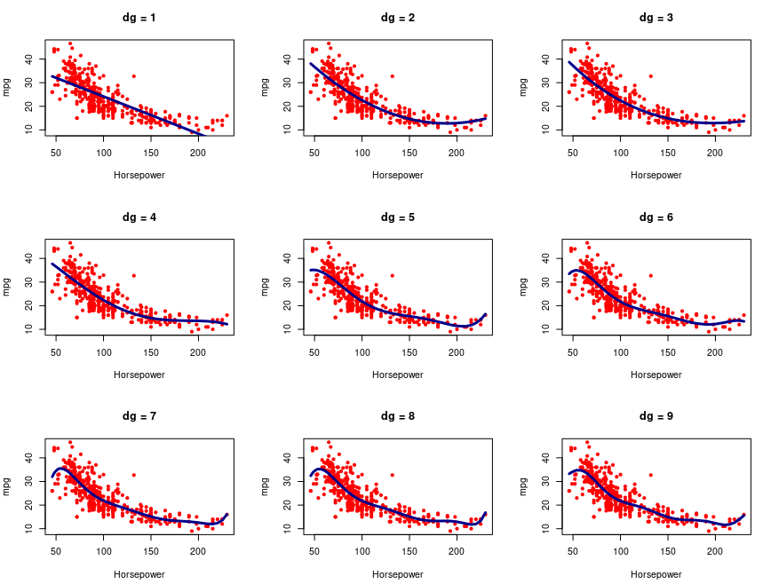
par(mfrow=c(3,3))
for (k in 1:length(dg)) {
g <- lm(mpg ~ poly(horsepower, dg[k]))
plot(mpg~horsepower, col=2, pch=20, xlab="Horsepower",
ylab="mpg", main=paste("dg =", dg[k]))
lines(horsepower[u], g$fit[u], col="darkblue", lwd=3)
}

# Single Split
set.seed(1)
n <- nrow(Auto)

# training set
tran <- sample(n, n/2)
MSE <- NULL
for (k in 1:length(dg)) {
    g <- lm(mpg ~ poly(horsepower, dg[k]), subset=tran)
    MSE[k] <- mean((mpg - predict(g, Auto))[-tran]^2)
}

# Visualization MSE_test
plot(dg, MSE, type="b", col=2, xlab="Degree of Polynomial",
ylab="Mean Squared Error", ylim=c(15,30), lwd=2, pch=19)
abline(v=which.min(MSE), lty=2)
3. K-fold Cross Validation
- K-fold Cross-validation divide the data into K equal-sized parts. We leave out part \(K\), fit the model to the other \(K - 1\) parts, and then obtain prediction for the left-out kth part.
- If we evaluate 10 models with 5-fold CV, then we need to consider \(5 \times 10\) cross validation score.
- We compare the average mean score of K cross validation scores among models.
- \(CVE = \frac{1}{n}\sum_{k=1}^{K}(n_k MSE_k)\)

# 10-fold cross validation
k <- 10
# degree is 1:9
MSE <- matrix(0, n, length(dg))
## MSE <- matrix(0, k, length(dg))

# Assertion each data point to each fold
# e.g. [1, 3, 3, 5, 6, ..., 10] (n)
set.seed(1234)
u <- sample(rep(seq(K), lengnth=n))

# Model training
"""
 f1     f2 f3 f4 f5 ... f9
MSE1
MSE2
...
MSE10
"""
for (k in 1:K) {
    tran <- which(u!=k)
    test <- which(u==k)
    for (i in 1:length(dg)) {
        g <- lm(mpg ~ poly(horsepower, i), subset=tran)
        MSE[test, i] <- (mpg - predict(g, Auto))[test]^2
        ## MSE[k, i] <- mean((mpg - predict(g, Auto))[test]^2)
    }
}
CVE <- apply(MSE, 2, mean)
## CVE <- apply(MSE, 2, mean)

# Visualization
plot(dg, CVE, type="b", col="darkblue",
xlab="Degree of Polynomial", ylab="Mean Squared Error",
ylim=c(18,25), lwd=2, pch=19)
abline(v=which.min(CVE), lty=2)
- The best parameter of degree of freedom is 2 when we consider inferring on population sets.
- This is elbow point of CVE plot.
4. LOOCV
Setting \(K = n\) yields leave-one-out cross validation(LOOCV).
# Auto Data : LOOCV
# Set the degree of freedom and result matrix
n <- nrow(Auto)
dg <- 1:9
MSE <- matrix(0, n, length(dg))

for (i in 1:n) {
    for (k in 1:length(dg)) {
        g <- lm(mpg ~ poly(horsepower, k), subset=(1:n)[-i])
        MSE[i, k] <- mean((mpg - predict(g, Auto))[i]^2)
    }
}
# Calculate CVE
aMSE <- apply(MSE, 2, mean)

# Visualization
par(mfrow=c(1, 2))
plot(dg, aMSE, type="b", col="darkblue",
     xlab="Degree of Polynomial", ylab="Mean Squared Error",
     ylim=c(18,25), lwd=2, pch=19)
abline(v=which.min(aMSE), lty=2)'Data Science > R' 카테고리의 다른 글
| [R] Best Subset Selection (0) | 2022.10.05 |
|---|---|
| [R] Linear Model (0) | 2022.10.05 |
| [R] Assessing Model Accuracy (0) | 2022.10.05 |
| [R] Flexibility and Interpretability (0) | 2022.10.05 |
| [R] Supervised Learning (0) | 2022.10.05 |


