[R] Supervised Learning

1. Model based on Supervised Learning

• Ideal model : \(Y = f(X) + \epsilon\)
• Good \(f(X)\) can make predictions of \(Y\) at new points \(X = x\).
• Statistical Learning refers to a set of approaches for estimating the function \(f(X)\).  

 

# Indexing without index
AD <- Advertising[, -1]

# Multiple linear regression 
lm.fit <- lm(sales ~. AD) 
summary(lm.fit) 
names(lm.fit) 
coef(lm.fit) 
confint(lm.fit) 

# Visualizing models 
par(mfrow=c(2,2))
plot(lm.fit) 

dev.off() 
plot(predict(lm.fit), residual(lm.fit)) 
plot(predict(lm.fit), rstudent(lm.fit)) 
plot(hatvalues(lm.fit))
which.max(hat.values(lm.fit))

 

2. Estimation of \(f\) for Prediction

• \(\hat{Y} = \hat{f}(X)\)
• \(\hat{f}\) : Estimation for \(f\).
• \(\hat{Y}\) : Prediction for \(Y\).
• Ideal function \(f(X)\) is \(f(X) = E(Y|X=x)\).
• Reducible error : \(E[(f(x) - \hat{f}(x))^2]\)
• Irreducible error : \(\epsilon = Y - f(x)\)
• Statistical learning techniques for estimating \(f\) is minimizing reducible error. 
• Statistical learning is the way finding \(\hat{f}\) which is the most similar function to \(f\).

 

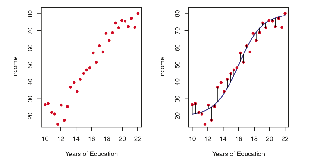
3. [Ex] Income Data

 

# Load Datasets 
url.in <- "https://www.statlearning.com/s/Income1.csv"
Income <- read.csv(url.in, h=T)

# Polynomial regression fit 
par(mfrow = c(1,2)) 
plot(Income~Education, col=2, pch=19, xlab="Years of Education", 
     ylab="Income", data=Income) 

g <- lm(Income ~ ploy(Education, 3), data=Income) 
plot(Income~Education, col=2, pch=19, xlab="Years of Education", 
     ylab="Income", data=Income)
lines(Income$Education, g$fit, col="darkblue", lwd=4, ylab="Income", 
      xlab="Years of Education")
      
# Compare residuals 
y <- Income$Income
mean((predict(g) - y)^2) 
mean(residuals(g)^2)

 

 

# Polynomial fit with multiple hyperparameter 
dist <- NULL
par(mfrow=c(3,4)) 
for (k in 1:12) { 
    g <- lm(Income ~ poly(Education, k), data=Income) 
    dist[k] <- mean(residual(g)^2)
    plot(Income~Education, col=2, pch=19, xlab="Years of Education", ylab="Income",
         data=Income, main=paste("k =", k)) 
    lines(Income$Education, g$fit, col="darkblue", lwd=3, ylabe="Income", xlab="Years of Education")
}

 

 

x11()
plot(dist, type="b", xlab="Degree of Polynomial", 
     ylab="Mean squared distance")