[R] Assessing Model Accuracy

1. How do we assess model accuracy? 

• Quantitative : MSE(mean squared error) 
• Qualitative : Classification error rate 
• Type of dataset
  • Training set : To fit statistical learning models
  • Validation set : To select optimal tuning parameter 
  • Test set : To select the best model 

 

2. MSE(Mean Squared Error) 

• Suppose our fitted model \(\hat{f}(x)\) from training dataset, \((x_i, y_i)\). 
• \(MSE_{train} = \frac{1}{n_1}\sum_{i \in {train}}[y_i - \hat{f}(x_i)]^2\)
• \(MSE_{test} = \frac{1}{n_2}\sum_{i \in {test}}[y_i - \hat{f}(x_i)]^2\)
• The best \(\hat{f}(x)\) is model which minimize \(MSE_{test}\).

 

3. [Ex] Cubic Model MSE 

# Simulate x and y based on a known function
set.seed(12345)
fun1 <- function(x) -(x-100)*(x-30)*(x+15)/13^4+6
x <- runif(50,0,100)
y <- fun1(x) + rnorm(50)

# Plot linear regression and splines
par(mfrow=c(1,2))
plot(x, y, xlab="X", ylab="Y", ylim=c(1,13))
plot(x, y, xlab="X", ylab="Y", ylim=c(1,13))
lines(sort(x), fun1(sort(x)), col=1, lwd=2)
abline(lm(y~x)$coef, col="orange", lwd=2)
lines(smooth.spline(x,y, df=5), col="blue", lwd=2)
lines(smooth.spline(x,y, df=23), col="green", lwd=2)
legend("topleft", lty=1, col=c(1, "orange", "blue", "green"),
legend=c("True", "df = 1", "df = 5", "df =23"),lwd=2)

# Simulate training and test data (x, y)
set.seed(45678)
tran.x <- runif(50,0,100)
test.x <- runif(50,0,100)
tran.y <- fun1(tran.x) + rnorm(50)
test.y <- fun1(test.x) + rnorm(50)

# Compute MSE along with different df
df <- 2:40
MSE <- matrix(0, length(df), 2)
for (i in 1:length(df)) {
    tran.fit <- smooth.spline(tran.x, tran.y, df=df[i])
    MSE[i,1] <- mean((tran.y - predict(tran.fit, tran.x)$y)^2)
    MSE[i,2] <- mean((test.y - predict(tran.fit, test.x)$y)^2)
}

# Plot both test and training errors
matplot(df, MSE, type="l", col=c("gray", "red"),
xlab="Flexibility", ylab="Mean Squared Error",
lwd=2, lty=1, ylim=c(0,4))
abline(h=1, lty=2)
legend("top", lty=1, col=c("red", "gray"),lwd=2,
legend=c("Test MSE", "Training MSE"))
abline(v=df[which.min(MSE[,1])], lty=3, col="gray")
abline(v=df[which.min(MSE[,2])], lty=3, col="red")

 

 

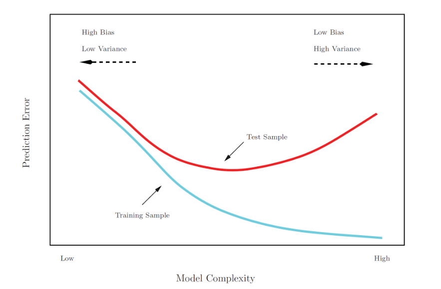
• red curve : \(MSE_{test}\)
• grey curve : \(MSE_{train}\)
•  \(MSE_{train}\) always decrease in every degree of flexiblity 
• \(MSE_{test}\) decrease if flexbility goes to optimal value of flexibility and increase when flexibility pass the optimal value. 

 

4. Bias Variance Trade-Off 

 

• Bias is an error from erroneuos assumptions in the learning algorithm. High bias can cause an algorithm to miss the relevant relations between features and target outputs. 
• Variance is an error from sensitivity to small fluctuations in the training set. High variance may result from an algorithm modeling the random noise in the training data. 
• If flexibility increases, Variance increases, Bias decreases. 
• If flexibility decreases, Variance decreases, Bias increases. 
• The best performance of a statistical learning methods : Low Bias + Low Variance 
• For the best performance of a statistical learning methods, we need to set model whch minimize \(MSE_{test}\).