1. Regression Decision Tree
1.1 [Ex] Finding optimal value
# Import library and dataset
library(tree)
data(Hitters)

# Training models
miss <- is.na(Hitters$Salary)
g <- tree(log(Salary) ~ Years + Hits + RBI + PutOuts + Walks + Runs + Assists + HmRun + Errors + Atbat, subset=!miss, Hitters)

# Perform 6 fold CV
set.seed(1234)
cv.g <- cv.tree(g, K=6)
plot(cv.g$size, cv.g$dev, type="b")

1.2 Workflow of optimizing unpruned tree
- Make tree model using tree function : g <- tree(format, subset=train, data)
- Perform K-fold CV using cv.tree function : cv.g <- cv.tree(tree, K=k)
- Find optimized tree size : w <- which.min(cv.g$dev)
- Prune tree using prune.tree function : g2 <- prune.tree(g, best=cv.g$size[w])
- Make prediction using predict function : yhat <- predict(g2, testset)
- Calculate MSE : sqrt(mean((yhat-tree.test)^2))
This is optimized model using metrics as 6-fold CV. The optimized alpha is stored in cv.g$size[w].
2. Calculating
2.1 MSE with using tree method
# Training sets and Test sets solitting
attach(Hitters)
newdata <- data.frame(Salary, Years, Hits, RBI, PutOuts, Walks, Runs, Assists, HmRun, Errors, AtBat)
newdata <- newdata[!miss, ]

# Separate samples into 132 training sets and 131 test sets
set.seed(1111)
train <- sample(1:nrow(newdata), ceiling(nrow(newdata)/2))

# Fit a tree with training set and compute test MSE
tree.train <- tree(log(Salary) ~ ., subset=train, newdata)
yhat1 <- exp(predict(tree.train, newdata[-train, ]))
tree.test <- newdata[-train, "Salary"]

# Visualize results
plot(yhat1, tree.test)
abline(0,1)
sqrt(mean((yhat1-tree.test)^2))

- xaxis : predicted values of regression decision tree
- yaxis : real vlaues of newdata[test]
- MSE : 376.4349
2.2 Using tree with optimized
# Perform 6 fold CV for training sets
set.seed(1234)
cv.g <- cv.tree(tree.train, K=6)
plot(cv.g$size, cv.g$dev, type="b")

# Prune a tree with training set and compute test MSE
# in the original sclae
w <- which.min(cv.g$dev)
prune.tree <- prune.tree(tree.train, best=cv.g$size[w])
yhat2 <- exp(predict(prune.tree, newdata[-train, ]))

# Visualize results
plot(yhat2, tree.test)
abline(0,1)
sqrt(mean((yhat2-tree.test)^2))

- MSE : 367.4892
2.3 Using Linear Regression using lm method
# Compute test MSE of least square estimates
g0 <- lm(log(Salary)~., newdata, subset=train)
yhat3 <- exp(predict(g0, newdata[-train,]))
sqrt(mean((yhat3-newdata$Salary[-train])^2))
- MSE : 407.3643
3. [Ex] Building Regression Decision Tree
Step 1 : Prerequirisite
library(MASS)
data(Boston)
str(Boston)
Step 2 : Training model with tree function on training set
# Train-test split
set.seed(1)
train <- sample(1:nrow(Boston), nrow(Boston)/2)

# Training models
tree.boston <- tree(medv ~ ., Boston, subset=train)
summary(tree.boston)

# Visualize results
plot(tree.boston)
text(tree.boston, pretty=0)

Step 3 : Training model with optimized
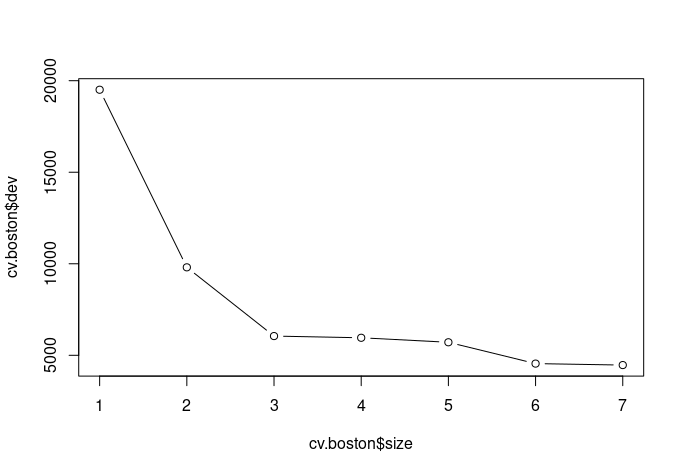
cv.boston <- cv.tree(tree.boston, K=5)
plot(cv.boston$size, cv.boston$dev, type="b")
which.min(cv.boston$dev)

Step 4 : Calculate MSE of tree model
# Make predictions
yhat <- predict(tree.boston, newdata=Boston[-train, ])
boston.test <- Boston[-train, "medv"]

# Visualize results
plot(yhat, boston.test)
abline(0, 1)

# Calculate MSE of test sets
mean((yhat - boston.test)^2)- MSE : 35.28688
Step 5 : Calculate MSE of linear regression model
g <- lm(medv ~ ., Boston, subset=train)
pred <- predict(g, Boston[-train,])
mean((pred - boston.test)^2)- MSE : 28.86123
Step 6 : Calculate MSE of regsubsets model
library(leaps)
g1 <- regsubsets(medv ~ ., data=Boston, nvmax=13, subset=train)
ss <- summary(g1)
cr <- cbind(ss$adjr2, ss$cp, ss$bic)
x.test <- as.matrix(Boston[-train, -14])
MSE <- NULL
for (i in 1:3) {
    beta <- rep(0, ncol(Boston))
    if (i > 1) ww <- which.min(cr[,i])
    else ww <- which.max(cr[,i])
    beta[ss$which[ww,]] <- coef(g1, ww)
    preds <- cbind(1, x.test) %*% beta
    MSE[i] <- mean((preds - boston.test)^2)
}
MSE- MSE of Adjusted R^2 : 26.85842
- MSE of AIC : 26.85842
- MSE of BIC : 29.10294
4. [Ex] Assignments
- The exhaustive variable selection method found 13 best models such that : summary(g1)$which[, -1]
- For each best model, fit a regression tree with the same training set and compute MSE of the same test set.
- Find the best model that minimize the test MSE among 13 models. Do not prune your regression tree.
# Importing Library
library(MASS)
data(Boston)
library(leaps)
library(tree)

# Train-Test Splitting
set.seed(1)
train <- sample(1:nrow(Boston), nrow(Boston)/2)

# Training model using regsubsets
g1 <- regsubsets(medv ~ ., data=Boston, nvmax=13, subset=train)

MSE <- NULL
for (i in 1:13) {
  x <- which(summary(g1)$which[i, -1] == 1)
  newdata <- data.frame(Boston[, c(x, 14)])
  tree.train <- tree(medv ~ ., newdata, subset=train)
  yhat <- predict(tree.train, newdata[-train, ])
  tree.test <- newdata[-train, "medv"]
  MSE[i] <- mean((yhat - tree.test)^2)
}
MSE

wm <- which.min(MSE)
wm- wm : 5
'Data Science > R' 카테고리의 다른 글
| [R] Tree-Based Methods : Advantages and Disadvantages of Tree (0) | 2022.11.27 |
|---|---|
| [R] Tree-Based Methods : Classification Decision Tree (1) | 2022.11.27 |
| [R] Tree-Based Methods : Decision Tree (0) | 2022.11.27 |
| [R] Non-Linear Models : Local Regression, GAM (0) | 2022.11.14 |
| [R] Non-Linear Models : Splines (0) | 2022.11.14 |


