1. Tree-Based Methods
- Tree-based methods for regression and classification involve stratifying or segmenting the predictor space into a number of simple regions
- The set of splitting rules used to segment the predictor space can be summarized in a tree.
- Tree-based methods are simple and useful for interpretation.
- Bagging and Random Forests grow multiple trees which are combined to yield a single consensus prediction.
- Combining a large number of trees can result in dramatic improvements in prediction accuracy, at the expense of some lose interpretation.
2. Decision Tree
- At a given internal node, the label (of the form (\(x_j < t_k\)) indicates the left-hand branch emanting from that split, and the right-hand branch corresponds to \(X_j \geq t_k\).
- The number in each leaf is the mean of the response for the observation that fall there.
2.1 [Ex] Decision Trees using tree package
# Import library and dataset
library(ISLR)
library(tree)
data(Hitters)
str(Hitters)

# Missing data
summary(Hitters$Salary)
miss <- is.na(Hitters$Salary)

# Fit a regression tree
g <- tree(log(Salary) ~ Years + Hits, subset=!miss, Hitters)
g
summary(g)

# Draw a tree
plot(g)
text(g, pretty=0)

tree(formula, data, weights, subsets, x, y)
A tree is grown by binary response partitioning using the response in the specified formula and choosing splits from the terms of the right-hand side.
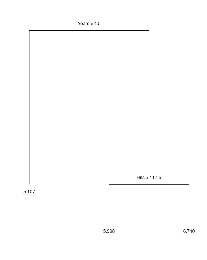
# Prune a tree
g2 <- prune.tree(g, best=3)
plot(g2)
text(g2, pretty=0)
prune.tree(tree, k=NULL, best=NULL, newdata)
Determine a nested sequence of subtrees of the supplied tree by recursively "snipping" off the least important splits.
- tree : fitted model object of class 'tree'.
- best : integer requesting the size of a specific subtree in the cost-complexity sequence to be returned.
2.2 [Ex] Decision Tree using rpart package
# Another R package for tree
library(rpart)
library(rpart.plot)

# Fit a regression tree
g3 <- rpart(log(Salary) ~ Years + Hits, subset=!miss, Hitters)
g3
summary(g3)

# Draw a fancy tree
prp(g3, branch.lwd=4, branch.col="darkgreen", extra=101)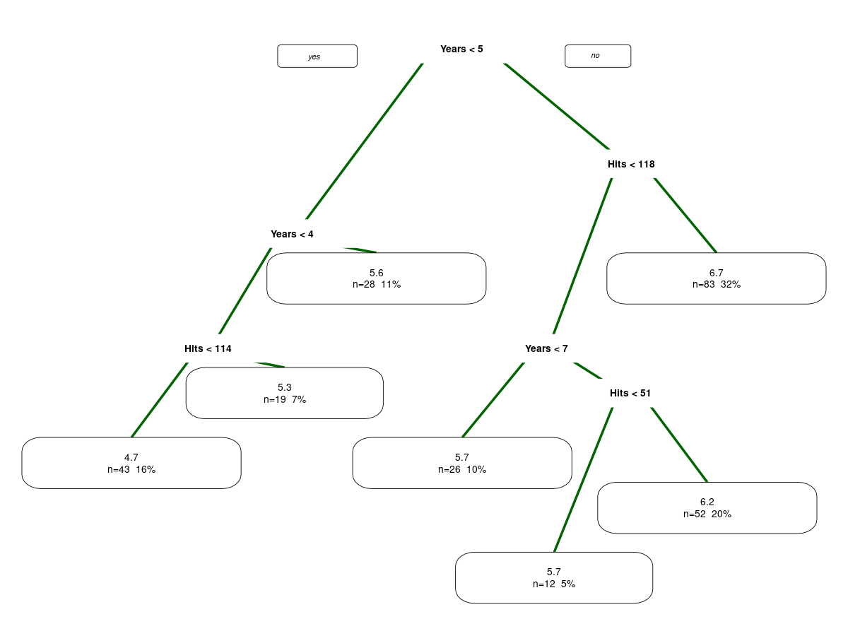
3. Details of the Tree-building Process
- Decision trees are typically drawn upside down, in the sense that the leaves are at the bottom of the tree.
- The points along the tree where the predictor space is split are referred to as internal node.
- The predictor space :
- Set of possible values : \(X_1, ..., X_p\)
- Non-overlapping regions : \(R_1, ..., R_j\)
- For every observation that falls into the region \(R_j\), make the same prediction which is simply the mean of the response value for the training observations in \(R_j\).
- Choose to divide the predictor space into high-dimensional rectangles.
The goal of constructing tree methods is finding boxes \(R_1, ..., R_j\) that minimizes the RSS(\(\sum_{j=1}^J\sum_{i\in R_j}(y_i - \hat{y}_{R_j})\)).
3.1 Recursive Binary Splitting
- Creating a binary decision tree is actually a process of dividing up the input space.
- A greedy approach is used to divide the space called recursive binary splitting.
- It is greedy because at each step of the tree-building process, the best split is made at that particular step rather than picking a split that will lead to a better tree in future step.
- Select the predictor \(X_j\) such that splitting the predictor space into the region {\(X|X_j < s\)} and {\(X|X_j \geq s\)} leads to the greatest possible reduction in RSS.
- Repeat the process, looking for the best predictor and best cutpoint in order to split the data further so as to minimize the RSS within each of the resulting regions.
- The process contiues until a stopping criterion is reached : no region contains more than five observations.
3.2 Pruning a Tree
- The process with many splits may produce good predictions on the training set, but is likely to overfit the data, leading poor testing set perfomance.
- A smaller tree with with fewer splits might lead lower variance and better interpretation at the cost of a little bias.
- Grow a very alrge tree \(T_0\), and then prune it back in order to obtain a subtree.
- Cost complexity pruning(weakest link pruning) : \(\sum_{m=1}^{|T|}\sum_{i:x_i \in R_m}(y_i - \hat{y}R_m)^2 + \alpha|T|\)
- \(\alpha\) controls a trade-off between the subtree's complexity and its fit to the training data.
- Selecting an optimal value \(\hat{\alpha}\) using Cross Validation.
3.3 Summary : Tree Algorithm
- Use recursive binary splitting to grow a large tree on the training data, stopping only when each terminal node has fewer than some minimum number of observations(stopping criterion).
- Apply cost complexity pruing to the large tree in order to obtain a sequence of best subtrees, as a function of \(\alpha\).
- We can use prune.tree(tree, best=K) function
- Use K-fold corss-validation to choos \(\alpha\). For each \(k = 1, ... K\) :
- Repeat step 1 and 2 on the \(\frac{K - 1}{K}\) th fraction of the training data, excluding the \(k\)th fold.
- Evaluate the mean squared prediction error on the data in the left-out \(k\) th fold, as a function of \(\alpha\).
- Average the results, and pick \(\alpha\) to minimize the average error.
- Return the subtree from step 2 that corresponds to the chosen value of \(\alpha\).
'Data Science > R' 카테고리의 다른 글
| [R] Tree-Based Methods : Classification Decision Tree (1) | 2022.11.27 |
|---|---|
| [R] Tree-Based Methods : Regression Decision Tree (0) | 2022.11.27 |
| [R] Non-Linear Models : Local Regression, GAM (0) | 2022.11.14 |
| [R] Non-Linear Models : Splines (0) | 2022.11.14 |
| [R] Non-Linear Models : Step Functions (0) | 2022.11.14 |


