1. What is Classification Problem?
1.1 Classification
- The response variable \(Y\) : Qualitative, Categorical
- feature vector \(X\) ~ qualitative response \(Y\) : \(C(X) \in C\)
- Interested in estimating the probabilities : \(P(Y=1|X) , P(Y=0|X)\)
1.2 [Ex] Credit Card Default Data
# Import Dataset
library(ISLR)
data(Default)
summary(Default)
attach(Default)

# Visualization of dataset
plot(income ~ balance, xlab="Balance", ylab="Income",
     pch=c(1,3)[unclass(default)],
     col=c("lightblue","red")[unclass(default)])

# Check the dataset with same sample size
set.seed(1234)
ss <- sample(which(default=="No"), sum(default=="Yes"))
ss <- c(ss, which(default=="Yes"))
us <- unclass(default[ss])
plot(income[ss] ~ balance[ss], xlab="Balance", pch=c(1,3)[us],
     col=c("lightblue","red")[us], ylab="Income")

# Boxplot of Default by Balance and Income
par(mfrow=c(1,2))
boxplot(balance~default, col=c("lightblue","red"), boxwex=0.5,
        xlab="Default", ylab="Balance")
boxplot(income~default, col=c("lightblue","red"), boxwex=0.5,
        xlab="Default", ylab="Income")
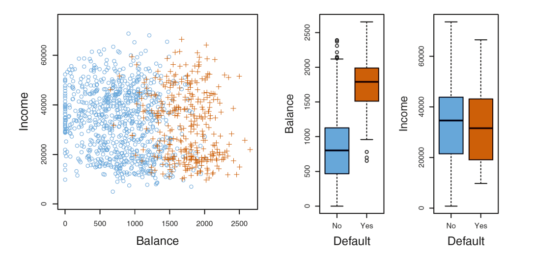
- Left : The annual incomes and monthly credit card balances of a number of individuals. Default(orange) and Not-default(blue)
- Right : Boxplots of either balance or income as a fnction of default status
2. Logistic Regression
- Probabilities : \(p(X) = Pr(Y=1|X) = \frac{\exp{\beta_0 + \beta_1 X}}{1 + \exp{\beta_0 + \beta_1 X}}\)
- Odds function: \(\log{\frac{p(X)}{1 - p(x)}} = \beta_0 + \beta X\)
- Estimate for \(p(X)\) lies between 0 and 1.
- Estimating parameters : Maximum likelihood function
- \(l(\beta_0, \beta) = \Pi_{i=1}^n (\frac{\exp{\beta_0 + x_i^T \beta}}{1 + \exp{\beta_0 + x_i^T \beta}})^y_i (\frac{1}{1 + \exp{\beta_0 + x_i^T \beta}})^{1-y_i}\)
2.1 [Ex] Basic Model with glm function
# Training model : balance
g2 <- glm(default ~ balance, family="binomial")
summary(g2)$coef

# Fitted values : The calculated probability
g2$fit

# Inverse logistic function : Calculating probability from new value
ilogit <- function(x, coef) {
      exp(cbind(1, x) %*% coef) / (1 + exp(cbind(1, x) %*% coef))
}
# Compared two values : This results will be same
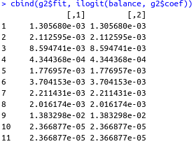
cbind(g2$fit, ilogit(balance, g2$coef))

# Calculate probability from new value x
ilogit(1000, g2$coef)
# 0.005751245
# Training model : student
g3 <- glm(default ~ student, family="binomial")
summary(g3)$coef

# Probability when student "yes"
ilogit(1, g3$coef)
# Probability when student "no"
ilogit(0, g3$coef)
- Student "yes" : 0.04313859
- Student "no" : 0.02919501
g4 <- glm(default ~ balance + income + student, family="binomial")
round(summary(g4)$coef, 4)
- Considering several variable in model at once, we can see that the value of studentYes is negative.
- This is because when we compare Default Rate in specific Balance between student or non-student, the rate of non-student is more higher than its of student.
2.1 [Ex] Find optimized model based on Validation Set
# Import library and dataset
library(glmnet)
library(ISLR)
data(Default)
attach(Default)

# Train-Test split
set.seed(1111)
n <- nrow(Default)
train <- sample(1:n, n*0.7)
test <- setdiff(1:n, train)

# Training model
g1 <- glm(default ~ balance, family="binomial", subset=train)
g2 <- glm(default ~ student, family="binomial", subset=train)
g3 <- glm(default ~ income, family="binomial", subset=train)
g4 <- glm(default ~ balance+student+income, family="binomial", subset=train)

# Testing model
miss <- NULL
for (k in 1:4) {
    g <- get(paste("g", k, sep=""))
    # Calculate probability from keyword "response"
    pred <- predict(g, Default, type="response")[test]
    ## yhat <- ifelse(pred > 0.5, 1, 0)
    yhat <- rep(0, length(test))
    yhat[pred > 0.5] <- 1
    miss[k] <- mean(yhat != as.numeric(default[test])-1)
}
miss

# result : 0.025000 0.0300000 0.030000 0.02366667
- Metric : Missclassification Error : mean(yhat != as.numeric(default[test]) - 1)
- We need to subtract 1 from default[test] (yes = 2, no = 1)
2.3 [Ex] Find optimized model based on K-fold CV
set.seed(1234)
K <- 10
n <- nrow(Default)
folds <- sample(rep(1:K, length=n))

miss <- rep(0, n)

for (k in 1:K) {
    train <- folds!=k
    test <- folds==k
    g <- glm(default ~ balance+student+income, family="binomial", subset=train)
    pred <- predict(g, Default, type="response")[test]
    yhat <- ifelse(pred > 0.5, 1, 0)
    miss[test] <- yhat != as.numeric(default[test])-1
}
mean(miss)

# 0.0289
3. Multinomial Logistic Regression
- \(Y \in {1, 2, ..., K}\)
- \(Pr(Y=k|X) = \frac{e^{\beta_{0k} + \beta_{1k}X_1 + ... \beta_{pk}X_p}}{\sum_{l=1}^{K} \beta_{0k} + \beta_{1k}X_1 + ... \beta_{pk}X_p }\)
- Only \(K-1\) linear functions are needed as in \(K\) class logistic regression.
3.1 [Ex] Wine dataset
# Importing library and dataset
# install.packages('remotes')
library(remotes)
install_github("cran/rattle.data")
library(rattle.data)
# install.packages('nnet')
library(nnet)
data(wine)

# Preview dataset wine
str(wine)
summary(wine)
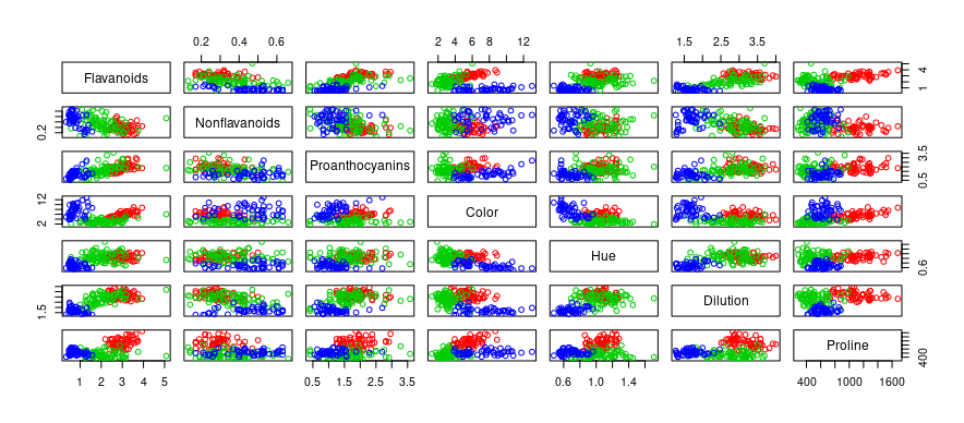
plot(wine[, -1], col=as.numeric(wine$Type) + 1)
plot(wine[, 2:7], col=as.numeric(wine$Type) + 1)
plot(wine[, 8:14], col=as.numeric(wine$Type) + 1)
# Fit model : Offers two coefficients
fit <- multinom(Type ~ ., data=wine, trace=FALSE)
summary(fit)

# Infer coefficients with Z-test
z <- coef(summary(fit))/summary(fit)$standard.errors
pnorm(abs(z), lower.tail=FALSE)*2
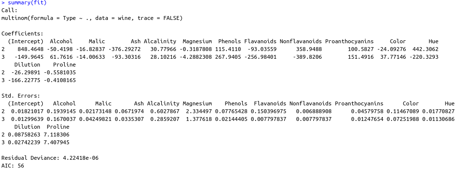

There are total two coefficients which divide three types of wine based on two decision boundary.
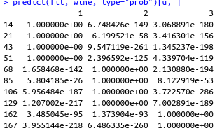
# Calculate conditional probability
set.seed(1)
u <- sort(sample(1:nrow(wine), 10))
fitted(fit)[u,]
predict(fit, wine, type="prob")[u, ]

# Predict based on probability
prob0 <- predict(fit, wine, type="prob")
pred0 <- apply(prob0, 1, which.max)
table(pred0, wine$Type)

# Predict based on class
pred0a <- predict(fit, wine, type="class")
table(pred0a, wine$Type)
3.2 Predict Classification result
- model$coef : Extract coefficients of trained model
- fitted(model) : Extract probability of training set
- predict(model, test_set, type="response") : predict probability in glm model
- yhat <- ifelse(pred > 0.5, 1, 0) : Class after calculating probability
- predict(model, test_set, type="prob") : predict probability of classification result
- yhat <- apply(prob0, 1, which.max) : Class after calculating probability
- predict(model, test_set, type="class") : predict class in multinom model
'Data Science > R' 카테고리의 다른 글
| [R] Assessment of the Performance of Classifier (0) | 2022.11.05 |
|---|---|
| [R] Classification Problem : LDA(Linear Discriminant Analysis) (0) | 2022.10.31 |
| [R] Elastic-Net Regression (0) | 2022.10.13 |
| [R] Regularization Methods (0) | 2022.10.11 |
| [R] Simulation Study : Prediction Performance (0) | 2022.10.11 |


