[R] Regularization Methods : Binary

1. Regulaization Methods

• Regularization methods are based on a penalized likelihood :
• \(Q_{\lambda}(\beta_0, \beta) = -l(\beta_0, \beta) + p_{\lambda}(\beta)\)
• \((\hat{\beta_0}, \hat{\beta}) = arg min Q_{\lambda}(\beta_0, \beta)\)
• Penalized likelihood for quantitive
  • Linear regression model : \(y_i = \beta_0 + x_i^T \beta + \epsilon_i\)
  • l1-norm : \(\lambda \sum(\hat{\beta}^2)\)
  • l2-norm : \(\lambda \sum|\hat{\beta}|\)
  • \(Q_{\lambda}(\beta_0, \beta) = -l(\beta_0, \beta) + p_{\lambda}(\beta) = \frac{1}{2}\sum_{i=1}^{n}(y_i - \beta_0 + x_i^T \beta)^2 +  p_{\lambda}(\beta)\)
•  Penalized likelihood for binary
  • CVE based on deviance : \(CVE = \frac{1}{n}\sum_{k=1}^K -2\sum_{i \in C_k}(y_i \log{\hat{p_i}^{[-k]} + (1 - y_i) \log{(1-\hat{p_i}^{[-k]})})} \)
  • if type="response" : \(p_i(\beta_0, \beta) = \frac{e^{\beta_0 + x_i^T \beta}}{1 + e^{\beta_0 + x_i^T \beta}}\)
  • CVE based on classification error : $CVE = \frac{1}{n}\sum\sum I(y_i - \hat{y_i})^{[-k]}$

 

2. [Ex] 2. Heart Data

# Importing Datasets 
library(glmnet)
url.ht <- "https://www.statlearning.com/s/Heart.csv"
Heart <- read.csv(url.ht, h=T)
summary(Heart)

# Preprocessing Data 
Heart <- Heart[, colnames(Heart)!="X"]
Heart[,"Sex"] <- factor(Heart[,"Sex"], 0:1, c("female", "male"))
Heart[,"Fbs"] <- factor(Heart[,"Fbs"], 0:1, c("false", "true"))
Heart[,"ExAng"] <- factor(Heart[,"ExAng"], 0:1, c("no", "yes"))
Heart[,"ChestPain"] <- as.factor(Heart[,"ChestPain"])
Heart[,"Thal"] <- as.factor(Heart[,"Thal"])
Heart[,"AHD"] <- as.factor(Heart[,"AHD"])
summary(Heart)
dim(Heart)
sum(is.na(Heart))
Heart <- na.omit(Heart)
dim(Heart)
summary(Heart)

# Train model 
## Logistic Regression
# Add dummy variable to original matrix x wihtout intercept 
x <- model.matrix(AHD ~., Heart)[,-1]
y <- Heart$AHD

# Train model 
g1 <- glmnet(x, y, family="binomial")

# Comparison lambda - coefficient, l1-norm - coefficient 
par(mfrow=c(1,2))
plot(g1, "lambda", label=TRUE)
plot(g1, "norm", label=TRUE)
df <- cbind(g1$lambda, g1$df)
colnames(df) <- c("lambda", "nonzero")
rownames(df) <- colnames(g1$beta)
df

 

 

• If lambda decreases, the number of active coefficients increase.
• If l1-norm increase(lambda decrease), the number of active coefficeints increase.

 

# Make evaluation : 10 folds 
set.seed(1234) 
K <- 10 
n <- length(y) 
fold <- sample(rep(1:K, length.out=n)) 
lam <- g1$lambda 
MSE <- matrix(0, n, length(lam)) 
for (i in 1:K) {
  test <- fold==i
  tran <- fold!=i 
  g <- glmnet(x[tran, ], y[tran], family="binomial", lambda=lam)
  prob <- predict(g, x[test, ], s=lam, type="response")
  yval <- y[test]=="Yes"
  MSE[test, ] <- -2*(yval*log(prob) + (1-yval)*log(1-prob))
}
CVE <- apply(MSE, 2, mean)

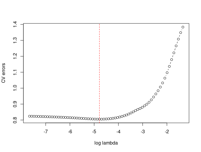
# Visualize CVE metrics 
par(mfrow=c(1,1))
plot(log(lam), CVE, type="b", xlab="log lambda", ylab="CV errors")
abline(v=log(lam)[which.min(CVE)], col="red", lty=2)

# Make final model : With full training set 
lam[which.min(CVE)]
coef(g, s=lam[which.min(CVE)])
g1 <- glmnet(x, y, family="binomial", lambda=lam[which.min(CVE)])
coef(g1)

 

 

• K-fold without using cv.glmnet.
• MSE has been used for model evaluation metrics.
• model.matrix function convert original data into categorical encoded columns and intercepts.
• To apply this metrx to glmnet, we need to input matrix without intercept.(beacuse inner argument of intercept is True).
• However, if we calculate prediction from the result of coef function, then we need to multiply with matrix with intercept.

 

3. [Ex] Heart Data with automatic CV

set.seed(123)
par(mfrow=c(1,3))
# Error metric : Deviance 
# foldID shows the restricted fold -> don't need to use nfolds parameters
gcv1 <- cv.glmnet(x, y, family="binomial", lambda=lam,
nfolds=5, type.measure="deviance")
plot(gcv1)

# Error metric : Classification error 
gcv2 <- cv.glmnet(x, y, family="binomial", lambda=lam,
nfolds=5, type.measure="class")
plot(gcv2)

# Error metric : ROC-AUC score
gcv3 <- cv.glmnet(x, y, family="binomial", lambda=lam,
nfolds=5, type.measure="auc")
plot(gcv3)

c(gcv1$lambda.min, gcv1$lambda.1se)
c(gcv2$lambda.min, gcv2$lambda.1se)
c(gcv3$lambda.min, gcv3$lambda.1se)
g0 <- glmnet(x, y, family="binomial", lambda=lam)
coef(g0, s=c(gcv1$lambda.min, gcv2$lambda.min, gcv3$lambda.min))
coef(g0, s=c(gcv1$lambda.1se, gcv2$lambda.1se, gcv3$lambda.1se))

 

 

• Three plots are written based on one-standard error.
• The left vertical line is the value of gcvl$lambda.min.
• The right vertical line is the value of gcvl$labmda.1se.