[Tensorflow] Stochastic Gradient Descent

1. The Loss Function

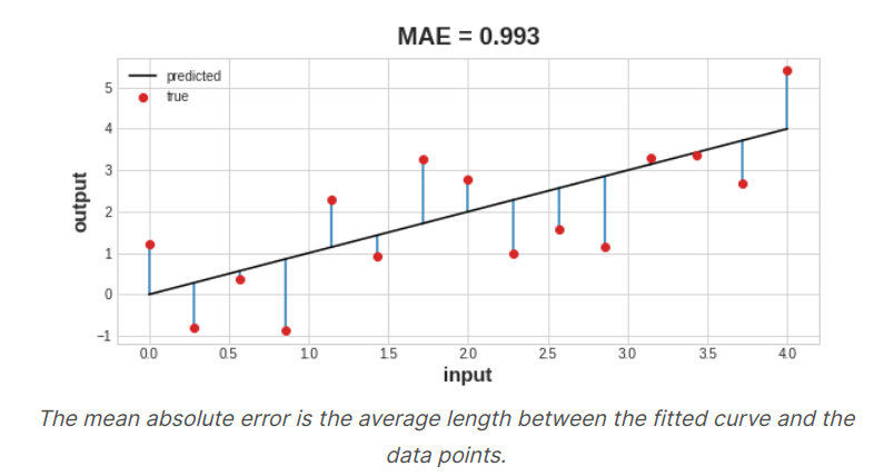
The loss function measures the disparity between the target's true value and the value the model predicts.

 

Different problems call for different loss functions. We've been looking at regression problems, where the task is predict some numerical value. A common loss function for regression problem is the mean absolute error or MAE. For each prediction y_pred, MAE measures the disparity from the true target y_true by an absolute difference \(abs(y_{true} - y_{pred}\). The total MAE loss on an dataset is the mean of all these absolute difference.

 

 

Besides MAE, other loss function we might see for regression problems are the mean_squared error(MSE) or the huber loss.

 

During training, the model will use the loss function as a guide for finding the correct value of its weights. In other words, the loss function tells the network its objective.

 

2. The Optimizer : Stochastic Gradient Descent

The optimizer is an algorithm that adjusts the weight to minimize the loss.

 

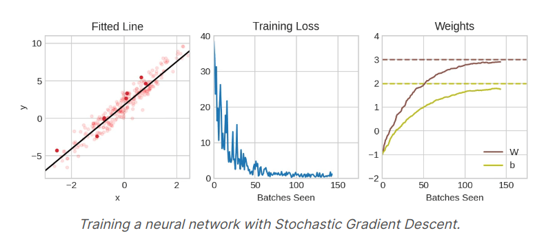
Virtually all of the optimization algorithms used in deep learning belong to a family called stochastic gradient descent. They are iterative algorithms that train a network in steps.

 

• Sample some training data and run it through the network to make predictions
• Measure the loss between the predictions and the true values
• Finally, adjust the weights in a direction that makes the loss smaller

Then just do this over and over until the loss is as small as we lilke. Each iteration's sample of training data is called mini batch while a complete round of the training data is called epoch. The number of epochs we train for is how many times the network will see each training example.

 

 

3. Learning Rate and Batch Size

Notice that the line only makes a small shift in the direction of each batch. The size of these shift is determined by the learning rate. A smaller learning rate means the network needs to see more mini batches before its weights converge to their best values.

 

The learning rate and the size of the mini batches are the two parameters that have the largest effect on how the SGD training proceeds. Their iteraction is often subtle and the right choice for these parameters isn't alwalys abvious.

 

Fortunately, for most work it won't be necessary to do an extensive hyperparameter searching to get satisfactory results. Adam is an SGD algorithm that has an adaptive learning rate that makes it suitable for most problems without any parameter tuning. Adam is great general-purpose optimizer.

 

4. Adding the Loss and Optimizer

import pandas as pd
from IPython.display import display
red_wine = pd.read_csv('../input/dl-course-data/red-wine.csv')

# Create training and validation splits
df_train = red_wine.sample(frac=0.7, random_state=0)
df_valid = red_wine.drop(df_train.index)
display(df_train.head(4))

# Scale to [0, 1]
max_ = df_train.max(axis=0)
min_ = df_train.min(axis=0)
df_train = (df_train - min_) / (max_ - min_)
df_valid = (df_valid - min_) / (max_ - min_)

# Split features and target
X_train = df_train.drop('quality', axis=1)
X_valid = df_valid.drop('quality', axis=1)
y_train = df_train['quality']
y_valid = df_valid['quality']


# Define a model 
from tensorflow import keras
from tensorflow.keras import layers

model = keras.Sequential([
    layers.Dense(512, activation='relu', input_shape=[11]),
    layers.Dense(512, activation='relu'),
    layers.Dense(512, activation='relu'),
    layers.Dense(1),
])

model.compile(
    optimizer='adam',
    loss='mae',
)

# This will show the changes of loss 
history = model.fit(
    X_train, y_train,
    validation_data=(X_valid, y_valid),
    batch_size=256,
    epochs=10,
)

# convert the training history to a dataframe
history_df = pd.DataFrame(history.history)

# use Pandas native plot method
history_df['loss'].plot();

 

 

Source from : https://www.kaggle.com/learn